부스팅 앙상블 (Boosting Ensemble) 3-1: XGBoost for Regression

이전 글 보기: 부스팅 앙상블 (Boosting Ensemble) 2-2: Gradient Boosting for Classification

이전 두 개의 포스팅에서 부스팅 앙상블의 초기 모델인 Gradient Boosting의 두 알고리즘 (Regression, Classification)에 대해 정리했습니다.
이번 포스팅에서는 최근 Kaggle에서 높은 점수를 기록하고 있는 XGBoost 알고리즘에 대해 정리해보겠습니다. Regression과 Classification 중 Regression 알고리즘을 먼저 다뤄봅니다.

XGBoost

XGBoost (eXtreme Gradient Boost)는 2016년 Tianqi Chen과 Carlos Guestrin 가 XGBoost: A Scalable Tree Boosting System 라는 논문으로 발표했으며, 그 전부터 Kaggle에서 놀라운 성능을 보이며 사람들에게 알려졌습니다.

XGBoost의 특징을 요약하면 아래와 같습니다.

1. Gradient Boost
2. Regularization
3. An unique regression tree
4. Approximate Greedy Algorithm
5. Parallel learning
6. Weighted Quantile Sketch
7. Sparsity-Aware Split Finiding
8. Cache-Aware Access
9. Blocks for Out-of-Core Computation

이 중 4-9번 항목은 알고리즘 효율성을 위한 최적화 방법을 나타내는 특징입니다. 지금은 개념을 익히는 중이니 일단 건너 뜁니다. 나중에 XGBoost Part 4: Crazy Cool Optimizations를 공부해서 정리해봅시다.

다시 돌아와서, 1번 Gradient Boost와 2번 Regularization은 별도의 포스팅을 통해 정리했습니다.

따라서 본 포스팅에서는 3번 unique regression tree의 과정을 정리해보고자 합니다. XGBoost Part 1: Regression를 참고했습니다.

XGBoost for Regression

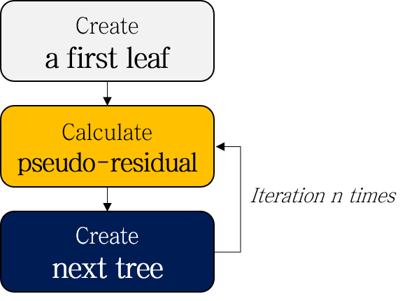
XGBoost for Regression은 Gradient Boosting for Regression과 전체적인 순서는 동일합니다. 샘플에 대한 residual을 계산하고, 이를 예측하는 decision tree를 만드는 과정을 반복한 뒤, learning rate \(\eta\)를 곱해 합칩니다.

다만 Step 3에서 몇 가지 차이점이 있습니다.

1. Create a first leaf
2. Calculate pseudo-residuals
3. Create next tree
   1. Similarity score of root node
   2. Separation based on Gain
   3. Complete decision tree with limitation of depth
   4. Prune the tree according to \(\gamma\)
   5. Calculate Output value (Representative value)
4. Repeat step 2-3

• (Test) Scale and add up the results of each tree

하나씩 차근차근 정리해봅시다.

예제 데이터입니다. XGBoost는 큰 데이터셋에 사용되는 모델이긴 하지만, 설명과 시각화의 편의를 위해 4개 샘플로 이루어진 데이터를 사용합니다.

1. Create a first leaf

다른 Boosting 알고리즘과 마찬가지로 A leaf로 모델을 시작합니다. 이 때 Leaf의 초기 예측값은 아무 숫자나 들어가도 되지만, 디폴트 값은 0.5를 사용합니다.

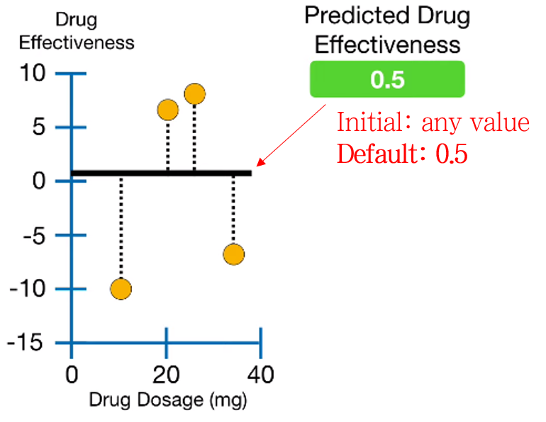
2. Calculate pseudo-residuals

실제값과 예측값의 차이인 Pseudo-residual을 계산합니다.

3. Create next tree

3-1. Similarity score of root node

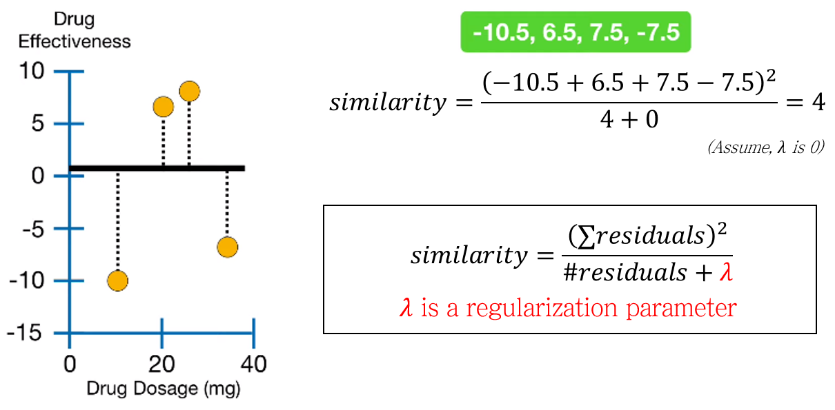
root node의 similarity score를 계산합니다. Similarity score는 아래와 같이 정의됩니다.

\[ Similarity\; score=\frac{sum\; of\; residuals^2}{the\; number\; of\; residuals+\lambda} \]

\(\lambda\)는 regularization score로, 0 이상의 값을 가집니다. \(\lambda\)가 XGBoost에 주는 영향은 후술하도록 하고, 일단 넘어갑니다.

3-2. Separation based on Gain

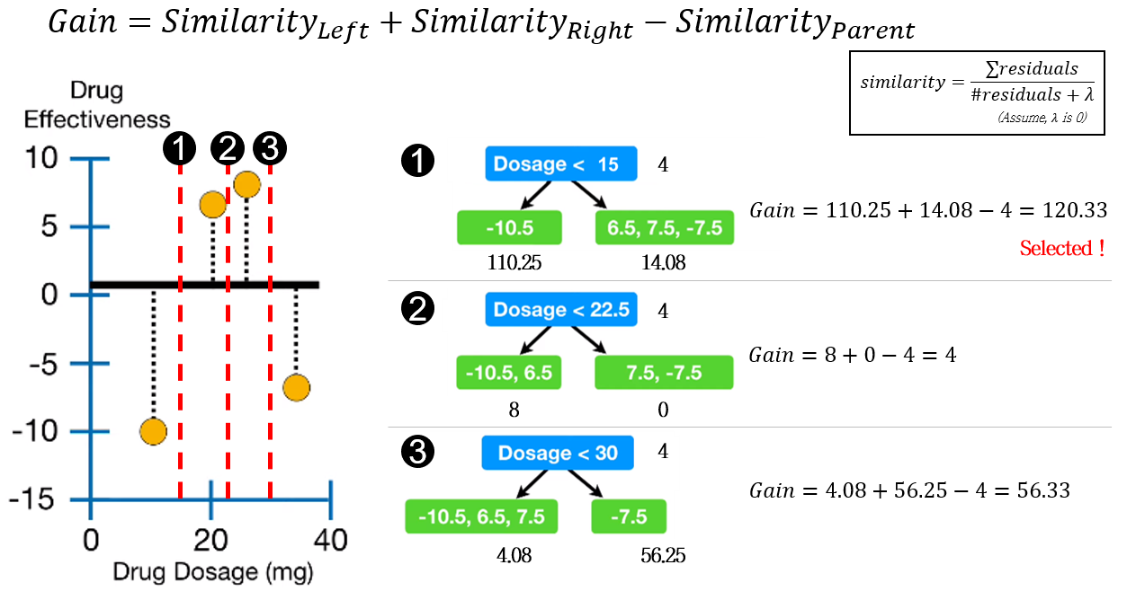
XGBoost에서 decision tree의 분기는 가장 큰 Gain 값을 갖는 지표로 이루어집니다. Gain은 아래와 같이 부모 노드와 자식노드의 Similarity score의 차로 계산됩니다.

\[ Gain=Similarity_{Left} + Similarity_{Right} - Similarity_{Parent} \]

위 예시에서는 1번 분기점이 가장 큰 Gain 값 (120.33)을 가지므로, Dosage < 15 조건으로 분기합니다.

3-3. Complete decision tree with limitation of depth

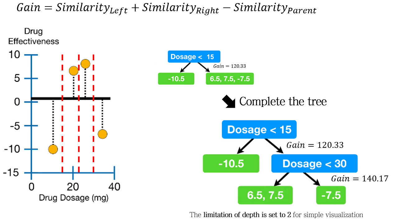
분기를 반복하여 decision tree를 완성시킵니다.

이 때, limitation of depth (나무의 깊이) 조건에 따라 tree가 만들어집니다. (디폴트 값은 6이지만, 예시에서는 시각화를 위해 2로 설정하여 만들었습니다.)

3-4. Prune the tree according to \(\gamma\)

다음 과정은 과적합 방지를 위한 가지치기 (pruning)입니다.

새로운 파라미터 \(\gamma\) 가 등장합니다. 각 분기지점에서 \(Gain-\gamma\)를 계산하여, 이 값이 음수일 때는 가지치기를 수행합니다 (해당 분기를 진행하지 않습니다).

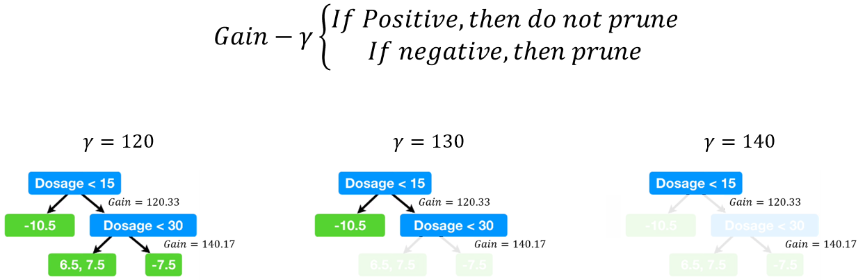
\(\gamma\) 가 120 / 130 / 140일 때의 가지치기 결과입니다.

3-5. Calculate Output value (Representative value)

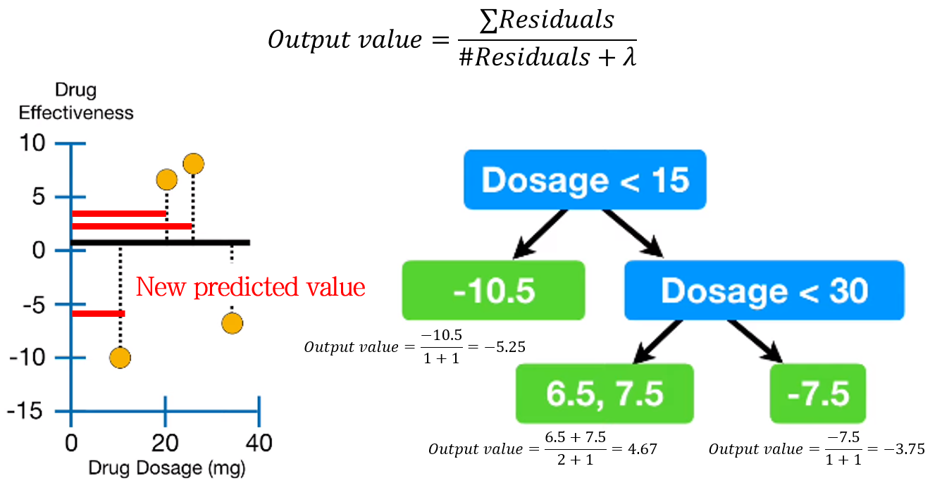
가지치기까지 끝난 decision tree의 각 leaf에 대한 output value (representative value)를 계산합니다. Output value 수식은 Similarity score와 비슷합니다 (분자가 square가 아닌 차이)

\[ Output\; value=\frac{sum\; of\; residuals}{the\; number\; of\; residuals+\lambda} \]

각 샘플에 대해 새로운 예측값도 계산합니다.

4. Repeat step 2-3

Decision tree를 계속해서 만듭니다.

(Test) Scale and add up the results of each tree

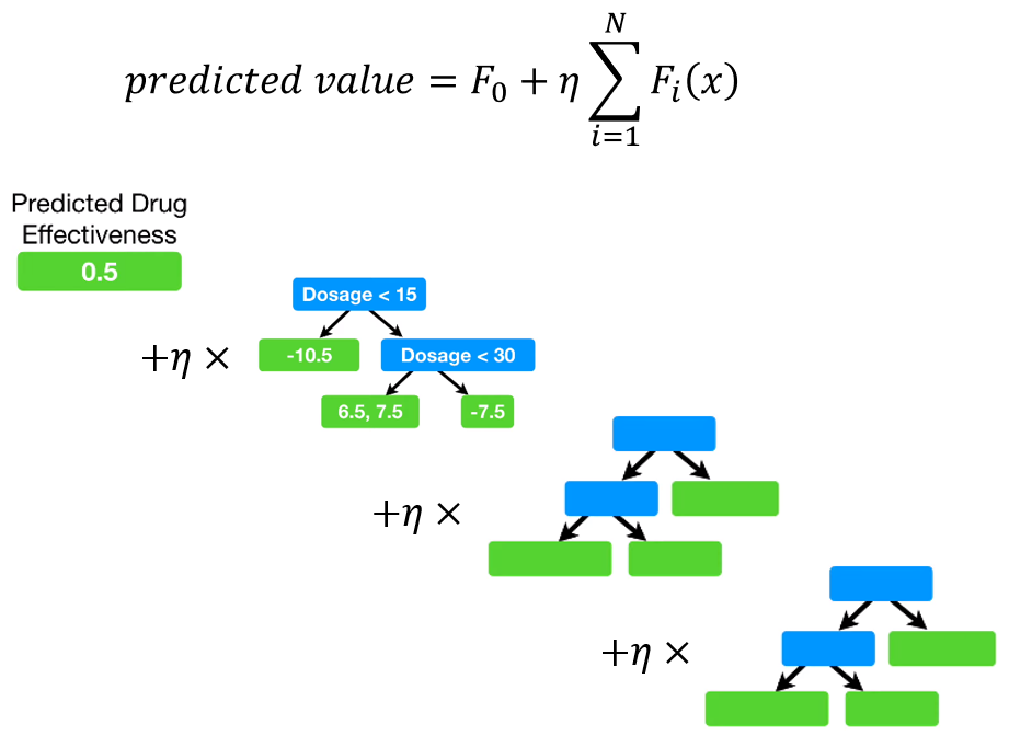
초기 예측값, 그리고 각 decision tree의 output value에 learning rate \(\eta\)를 곱한 값들을 다 더해 최종 예측값을 구합니다.

Properties of parameter \(\lambda, \gamma\)

Higher \(\lambda\) makes lower similarity score

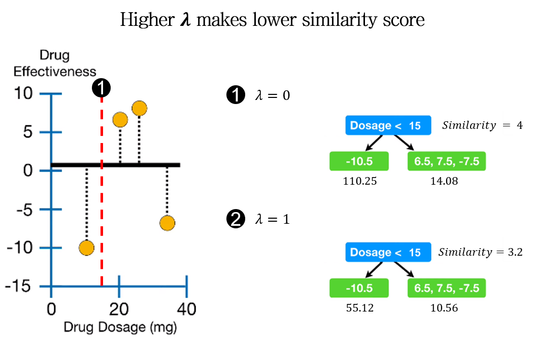
위 예시에서 \(\lambda\)의 값이 커짐에 따라 similarity가 작아지는 것을 확인할 수 있습니다. Similarity score의 분모에 \(\lambda\)가 있기 때문에, 반비례하는 특성을 갖습니다.

Higher \(\lambda\) makes more pruning

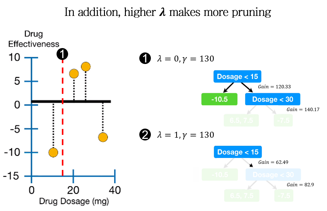
Similarity score의 감소는 Gain를 감소시킵니다. 따라서 더 낮은 \(\gamma\) 값에도 가지치기를 수행하게 됩니다.

결과적으로 \(\lambda\) 의 증가는 더 많은 가지치기를 수행하게 만듭니다.

\(\gamma=0\) does not mean turning off pruning

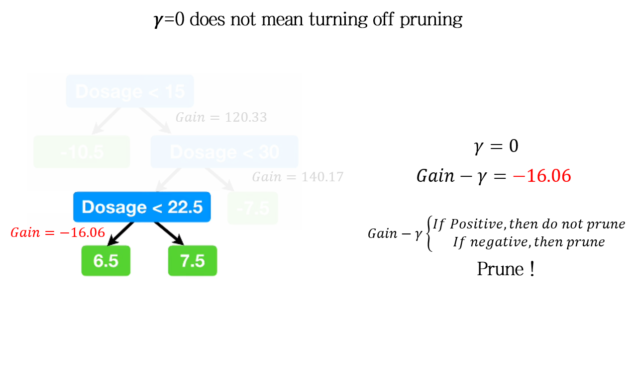
위 예시에서는 Gain 자체가 음수값을 갖습니다. 따라서, \(\gamma=0\)인 조건임에도 가지치기가 진행됩니다. 즉, \(\gamma=0\) 은 가지치기가 일어나지 않는다. 를 의미하는 것이 아닙니다.

Python code

Python 에서는 xgboost library로 사용 가능합니다.

• XGBoost Docs

관련 코드 추가 예정

---

다음 포스팅에서는 XGBoost 모델의 Classification 알고리즘을 정리해보도록 하겠습니다.

다음 글 보기: 부스팅 앙상블 (Boosting Ensemble) 3-2: XGBoost for Classification