부스팅 앙상블 (Boosting Ensemble) 3-2: XGBoost for Classification

이전 글 보기: 부스팅 앙상블 (Boosting Ensemble) 3-1: XGBoost for Regression

이전 포스팅에서는 XGBoost for Regression 알고리즘을 정리했습니다.
이번 포스팅에서는 XGBoost for Classification 알고리즘을 정리해보도록 하겠습니다.

XGBoost for Classification

XGBoost for Classification은 Gradient Boosting for Classification과 XGBoost for Regression에 대한 이해가 기본으로 깔려있어야 합니다. 두 내용을 모두 이해하고 있다면, 이번 포스팅은 이해하기 쉽습니다 😀

추가로 Odds와 Log(Odds)에 대한 이해도 필요합니다.

위의 알고리즘과 개념이 낯설다면 이전 포스팅들을 참고해주세요 !

XGBoost for Classification의 학습 과정은 XGBoost for Regression과 유사합니다. 다만 Gradient Boosting for Classification처럼 Probability의 residual을 예측하는 decision tree를 생성합니다.

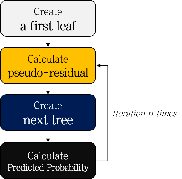
1. Create a first leaf
2. Calculate pseudo-residuals of probability
3. Create a next tree to predict pseudo-residuals
   1. Similarity score of root node
   2. Separation based on Gain
   3. Complete decision tree with limitation of limitation of depth
   4. Prune the tree according to \(\gamma\)
   5. Calculate Output value (Representative value)
4. Calculate predicted probability
5. Repeat step 2-4

• (Test) Scale, add up the results of each tree, and convert to probability

XGBoost for Regression과 전체적인 흐름이 거의 비슷하지만, Step 4가 추가된 것을 볼 수 있습니다. 예제 데이터로 전 과정을 천천히 정리해봅시다.

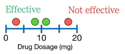
설명에 사용될 예시 데이터입니다. Drug dosage에 따라 약이 효과적일지 구분하는 binary classificatio문제로, 총 4개의 샘플이 있습니다.

1. Create a first leaf

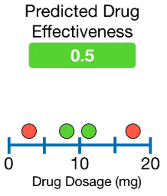
XGBoost for Classification에서도 여느 Gradient Boosting처럼 leaf로 시작합니다. leaf의 예측값은 drug가 효과적일지 맞추는 확률값으로, 디폴트 값은 0.5입니다.

2. Calculate pseudo-residuals of probability

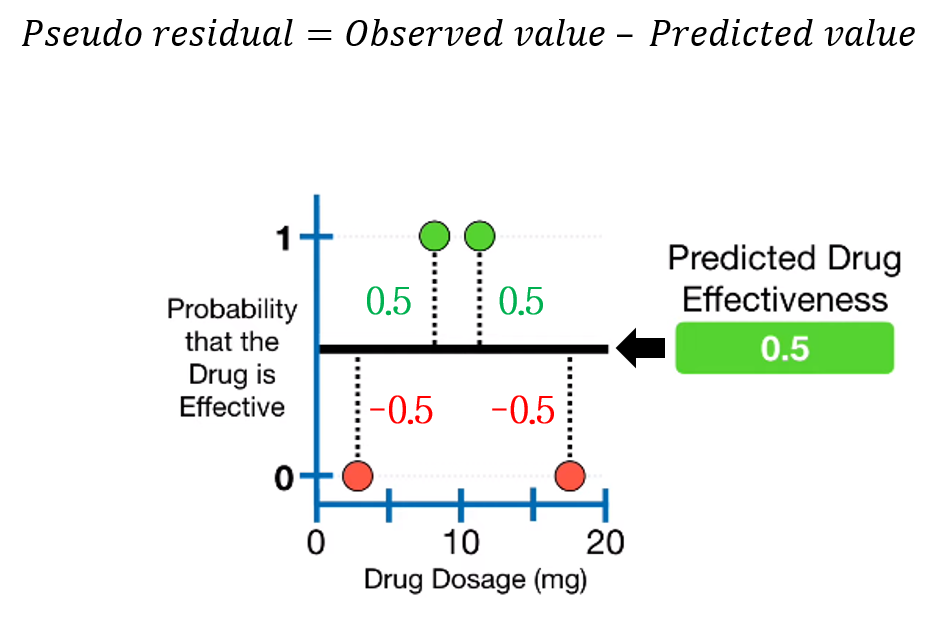
첫 leaf 모델의 예측값이 정해졌으니, 실제값 - 예측값, 즉 pseudo-residual을 계산할 수 있습니다. Gradient Boosting for Classification에서와 동일하게, Probability의 residual을 계산합니다.

3. Create a next tree to predict pseudo-residuals

3-1. Similarity score of root node

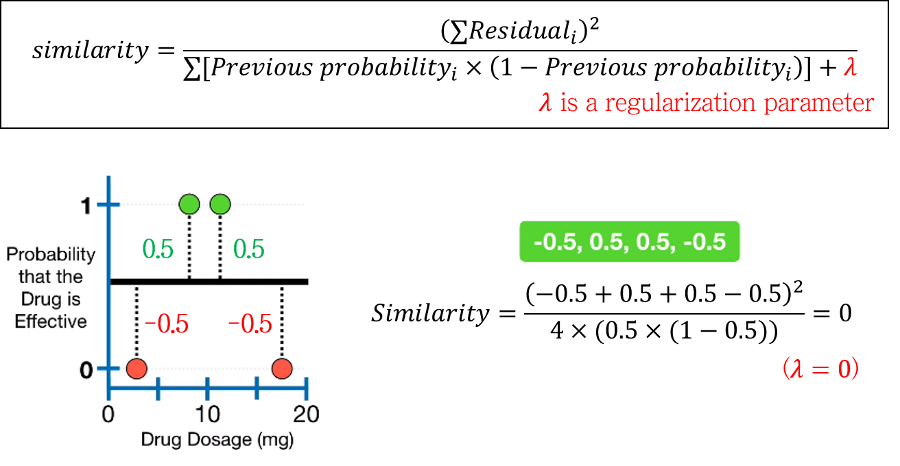
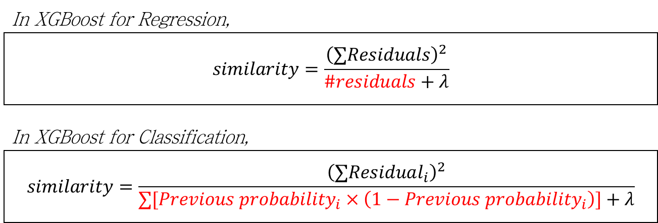
Similarity score가 다르게 정의됩니다. 복잡하게 생겼지만 XGBoost for Regression의 similarity score에서 분모부분만 바뀐 것을 확인할 수 있습니다. 바뀐 부분 또한 Gradient Boosting for Classification에서 본 log(odds) -> 확률 변환 수식과 비슷하게 생겼습니다.

\[ Similarity\; score=\frac{(\sum Residual_i)^2}{\sum[Previous\; probability_i \times (1-Previous\; probability_i)]+\lambda} \]

3-2. Separation based on Gain

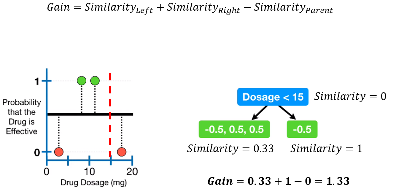
Gain의 정의는 동일합니다. 최대의 Gain을 갖는 분기 조건을 찾아 분기를 진행합니다.

3-3. Complete decision tree with limitation of limitation of depth

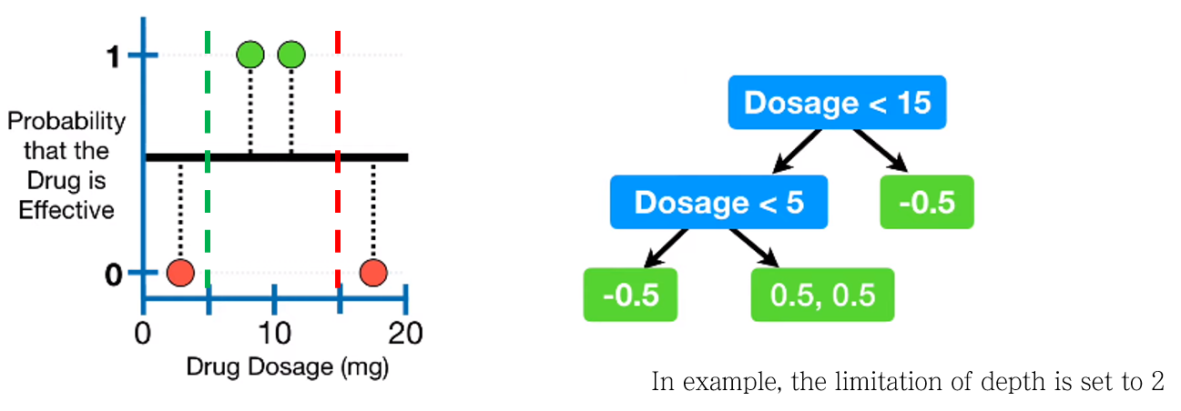
최적의 Tree를 완성했습니다. 예시에서는 limitation of depth 조건을 2로 셋팅했기 때문에 더 이상 분기하지 않습니다.

Depth 외에도 다른 조건을 걸 수 있습니다. 바로 min_child_weight 으로 사용되는 \(Cover\)라는 것입니다.

Cover 의 개념

Cover는 similarity score에서 분모 중 \(\lambda\)를 제외한 term을 의미합니다. 이 값이 \(Cover\) parameter 값보다 작을 경우, 해당 leaf는 가지치기를 수행합니다.

XGBoost for Regression에서는 \(Number\; of\; residuals\)이 크기 때문에 \(Cover\) 값이 커도 어느 정도 괜찮지만, Classification에서는 확률의 곱이다보니 \(Cover\) 에 따라 많은 leaf가 가지치기당하게 됩니다. 따라서 Classification에서는 \(Cover=0\) 으로 셋팅하는 것이 좋다고 합니다.

3-4. Prune the tree according to \(\gamma\)

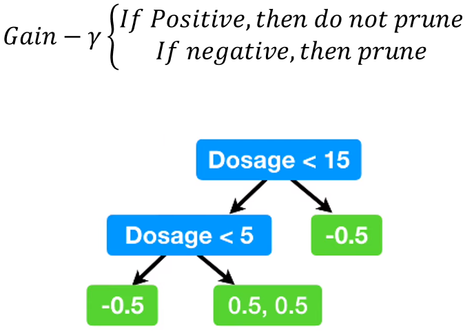
가지치기를 수행합니다. 예시에서는 모든 노드가 가지치기가 되지 않았습니다.

3-5. Calculate Output value (Representative value)

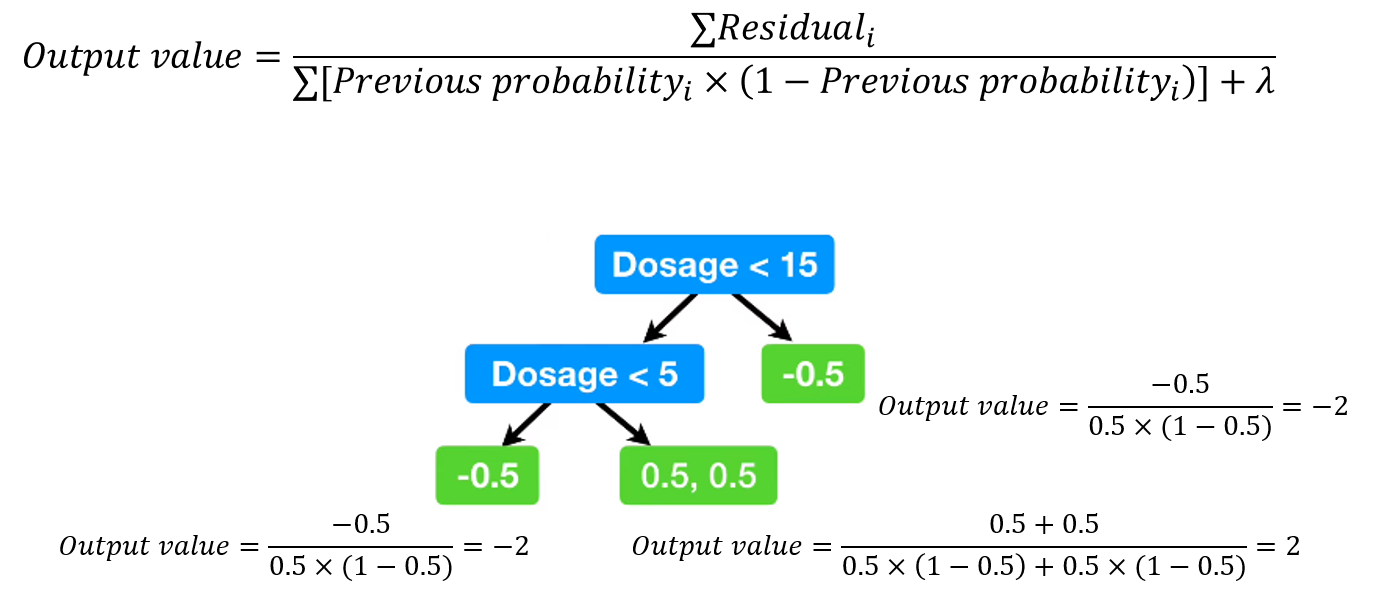
각 leaf에 대해 Output value (Representative value)를 계산합니다. Similarity score와 비슷하게 생긴 이 값은 log(odds)값으로 생각할 수 있습니다. 또한 Gradient Boosting의 output value 변환 식에서 \(\lambda\)만 추가된 식이기도 합니다.

\[ Output\; value=\frac{\sum Residual_i}{\sum[Previous\; probability_i \times (1-Previous\; probability_i)]+\lambda} \]

4. Calculate predicted probability

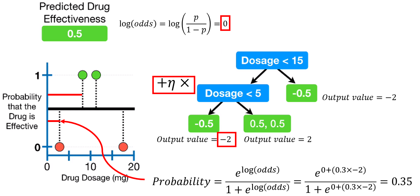
first leaf의 예측값도 확률값이었으니, log(odds)로 변환해줍니다. 그리고 각 모델의 log(odds)값에 learning rate \(\eta\)를 곱해 모두 합쳐줍니다.

마지막으로 다시 확률로 변환해주면 새로운 predicted probability를 얻을 수 있습니다.

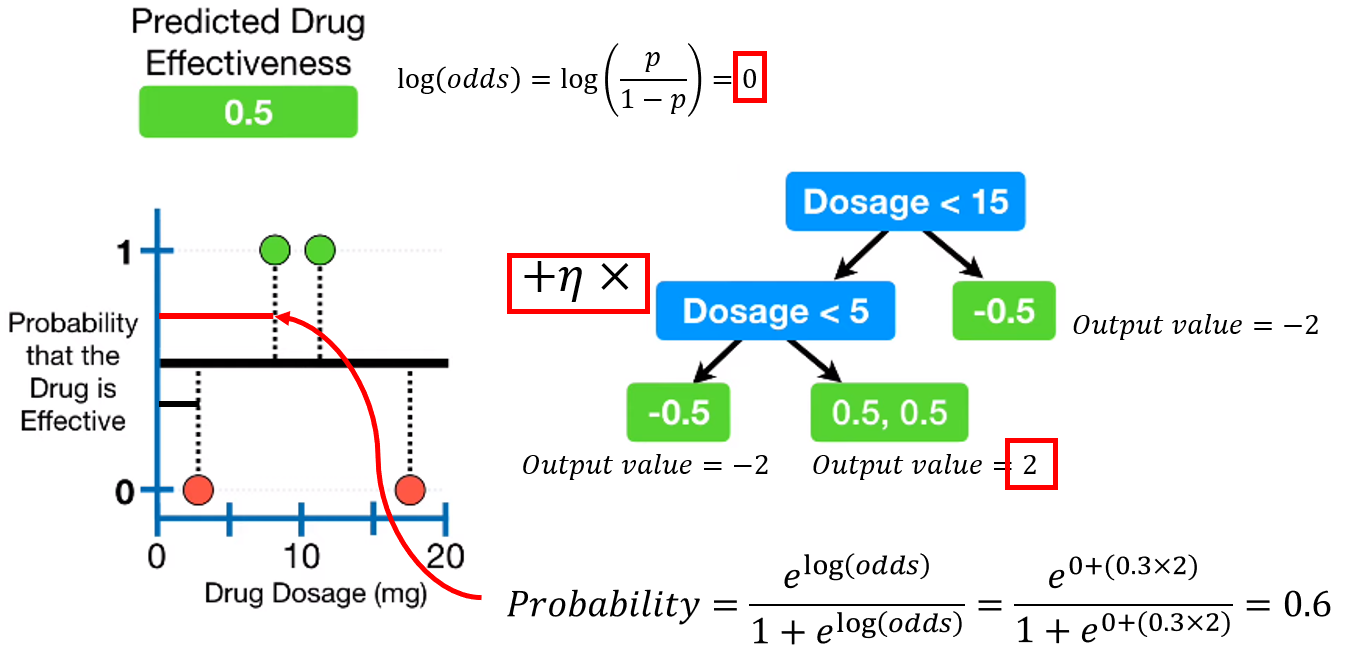
모든 샘플에 대해 이 과정을 수행합니다.

5. Repeat step 2-4

그리고 Tree의 생성을 계속해줍니다.

maximum number of tree에 도달하거나, Residual이 지정한 threshold 이하로 떨어지면 생성을 멈춥니다.

(Test) Scale, add up the results of each tree, and convert to probability

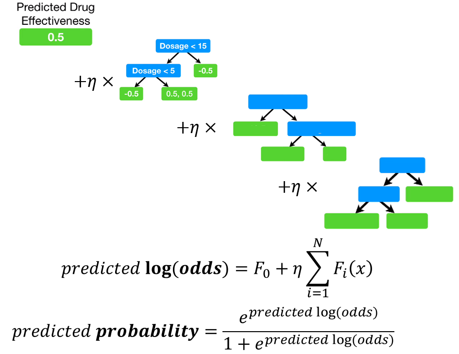
first leaf와 모든 tree의 log(odds)를 합친 후, probability로 변환하여 최종 예측값을 얻어냅니다.

Python code

Python 에서는 xgboost library로 사용 가능합니다.

• XGBoost Docs

---

다음 포스팅에서는 빠른 속도와 준수한 성능을 자랑하는 Microsoft의 LightGBM 모델에 대해 정리해보겠습니다.

다음 글 보기: 부스팅 앙상블 (Boosting Ensemble) 4: LightGBM